 Log In
Search




 Open Access
 lpdbyusst@163.com
Piding Li, School of Health Science and Engineering, University of Shanghai for Science and Technology, No. 516 Jungong Road, Yangpu District, Shanghai 200093, China. E-mail: lpdbyusst@163.com.
Received March 11, 2026; Accepted April 20, 2026; Published June 25, 2026
● A multi-frequency electromagnetic excitation scheme is proposed for the detection and localization of tiny metallic foreign bodies inside the human body.
● By integrating SHE-PWM with a full-bridge Class-D power amplifier, the transmitter achieves energy-efficient, spectrally controllable, and synchronous multi-frequency excitation.
Open Accesslpdbyusst@163.comPiding Li, School of Health Science and Engineering, University of Shanghai for Science and Technology, No. 516 Jungong Road, Yangpu District, Shanghai 200093, China. E-mail: lpdbyusst@163.com.
Received March 11, 2026; Accepted April 20, 2026; Published June 25, 2026
● A multi-frequency electromagnetic excitation scheme is proposed for the detection and localization of tiny metallic foreign bodies inside the human body.
● By integrating SHE-PWM with a full-bridge Class-D power amplifier, the transmitter achieves energy-efficient, spectrally controllable, and synchronous multi-frequency excitation.
Keywords: SHE-PWM, Class-D power amplifier, Eddy current testing, Balanced metal coil, Detecting tiny metal in body
In modern medical practice, inadvertent introduction and retention of metallic foreign bodies in the human body are not uncommon. Representative scenarios include accidental ingestion of metal fragments, traumatic retention of shrapnel or steel pellets, and intraoperative loss of small metallic items such as suture needles, hemostatic clips, guidewires, or miniature instrument components [1, 2]. Once retained, such foreign bodies may trigger localized inflammatory reactions, tissue injury, elevated infection risk, and even secondary harm during subsequent examinations or interventions. Accordingly, clinical management typically requires a prompt closed-loop workflow encompassing screening, localization, and retrieval. At present, X-ray radiography and computed tomography (CT) remain the mainstream modalities for metal localization, as they can directly depict the morphology of the foreign body and its spatial relationship with surrounding tissues. However, during perioperative or emergency management, physiological motions—including muscle contraction, respiration, and gastrointestinal peristalsis—can cause foreign-body migration; moreover, the use of X-ray or CT is often constrained by the size and limited maneuverability of these large-scale systems, which may delay screening and removal. Therefore, the development of a low-cost, portable, and real-time auxiliary localization technique capable of rapid confirmation and dynamic tracking beyond conventional imaging has clear engineering value and clinical significance.
Compared with conventional industrial metal detection, human-body metallic foreign-body detection is more challenging. Targets may be deeply embedded across different tissue layers with variable stand-off distance from the sensing coil. In addition, foreign bodies exhibit diverse morphologies (needle-like, plate-like, or particulate), and dynamic orientations driven by respiration, muscle contraction, and peristalsis. Meanwhile, biological tissues are conductive and dielectric with substantial inter-subject variability, and the presence of metallic surgical instruments further complicates the electromagnetic background and increases interference. Under such conditions, a single excitation frequency is often insufficient to satisfy both sensitivity and stability requirements. Hence, multi-frequency eddy-current techniques are desirable to improve detection efficiency: lower frequencies enhance effective penetration depth and facilitate detectability of deeply embedded objects, whereas higher frequencies strengthen near-surface responses and improve resolution for small or superficial targets, thereby improving reliability under complex backgrounds and posture variations [3, 4].
Eddy-current-based detection provides a feasible route for rapid localization of metallic foreign bodies in the human body. An excitation coil generates an alternating magnetic field that induces eddy currents in the metallic target (or magnetization responses in ferromagnetic objects) [5-7]. The resulting magnetic-field perturbation is then sensed by a receiving coil, enabling the determination of target presence and relative position. Similar to industrial in-line rejection systems, this approach relies on high-sensitivity acquisition and robust decision-making to detect weak electromagnetic signals.
The overall architecture of an eddy-current detection system is illustrated in Figure 1, typically comprising a power transmitter, a receiving and signal-conditioning front end, an analog-to-digital converter (ADC), and a digital processing unit (e.g., a microcontroller or field-programmable gate array [FPGA]). Among these components, the power transmitter is indispensable for improving the signal-to-noise ratio (SNR) and overall sensitivity: by delivering high-current excitation, it generates a sufficiently strong alternating electromagnetic field, thereby increasing the magnitude of target-induced field perturbations and the induced voltage at the receiver [8, 9]. In multi-frequency eddy-current detection, critical information is encoded in the frequency-dependent responses associated with target material properties, size, and depth. Therefore, the transmitter must provide not only high-power output but also synchronous, stable, and controllable multi-frequency excitation, ensuring phase coherence, amplitude consistency, and spectral purity across frequencies to meet the requirements of demodulation and feature extraction, and to avoid inter-frequency coupling and amplitude/phase drift that would otherwise degrade localization or identification accuracy. To this end, this work designs a synchronous multi-frequency transmitter employing a selective harmonic elimination (SHE) strategy to synthesize the excitation current waveform, enhancing the desired frequency components while suppressing non-target harmonics, thereby providing a stable transmission foundation for high-sensitivity detection under multi-frequency excitation.


Figure 2 schematically illustrates the operating principle of eddy-current–based detection. The output of the power amplifier drives the transmit coil. To enhance the coupling (sensing) coefficient between coils in the metal-detection probe, the transmit and receive coils are arranged in a coaxial coplanar configuration, with the transmit coil placed externally and the receive coil internally. The alternating magnetic field generated by the detection coil induces a rotational electric field in the conductive target, thereby driving closed-loop eddy-current distributions. According to Lenz’s law, these eddy currents generate a secondary magnetic field that couples back to the primary excitation field, thereby altering the magnetic flux linkage and the equivalent impedance of the detection coil [10, 11]. The resulting impedance variation comprises both a resistive component, associated with Joule losses induced by eddy currents, and an inductive component, associated with magnetic-flux redistribution (with explicit frequency dependence) [12, 13]. This impedance response is jointly governed by the target’s electrical conductivity and magnetic permeability, as well as its geometry, spatial position, and the excitation frequency (via the skin-depth effect). By measuring and demodulating the amplitude and phase of the coil voltage or current (or equivalently the in-phase and quadrature [I/Q] components), one can detect the presence of metallic targets and further enable parameter characterization, localization, and identification.
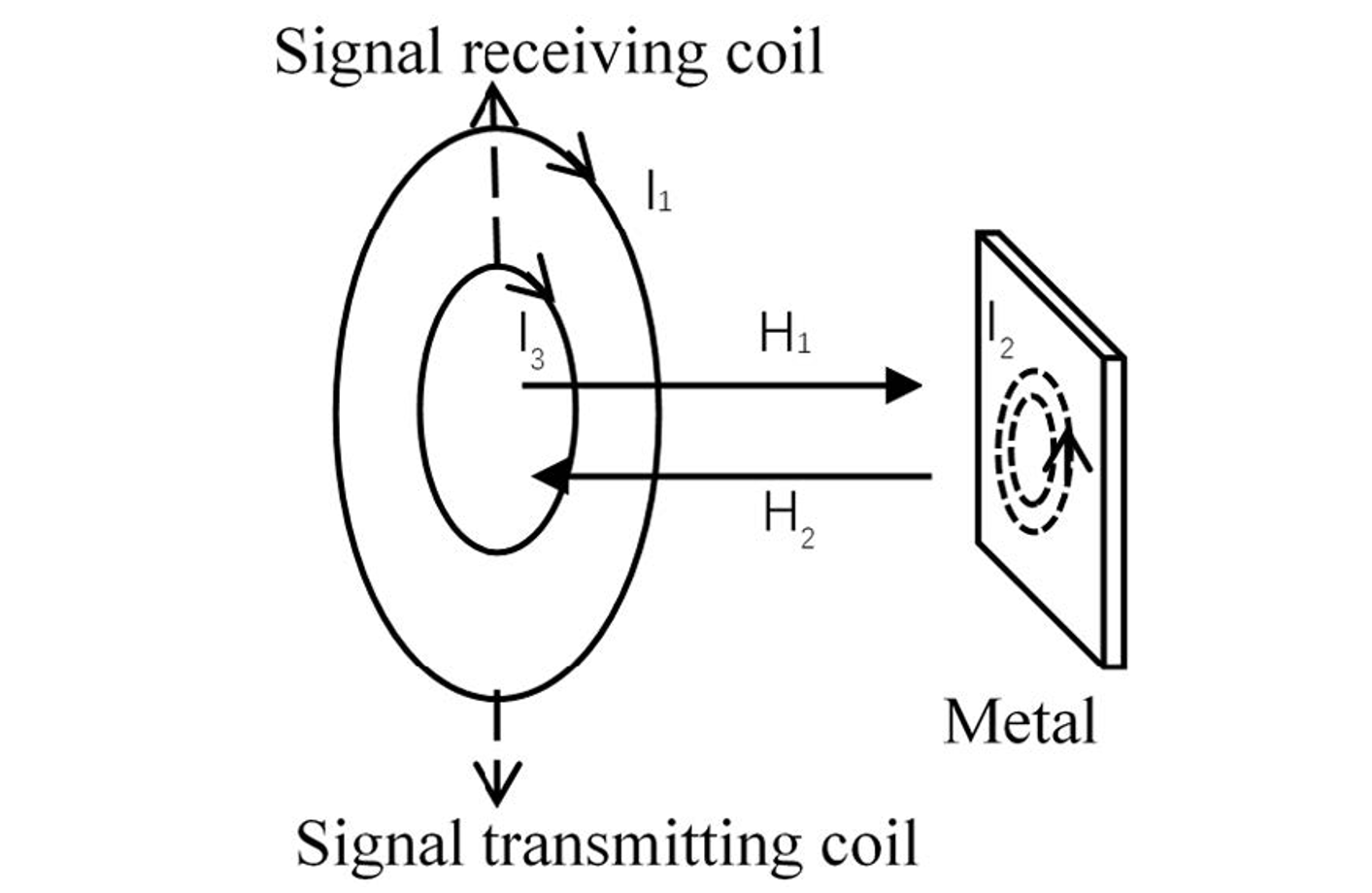
In the above-described electromagnetic detection system, the transmitting coil requires excitation currents of sufficiently high magnitude, making the choice of power amplifier configuration critical to overall system performance. For single-frequency eddy-current detection systems, a resonant driving scheme can be employed, in which the transmit coil and matching network form a resonant circuit capable of delivering power efficiently at a single frequency. However, for multi-frequency excitations, simultaneous resonance across multiple frequency components is impractical due to the inherently narrowband characteristics of resonant amplifiers.
In the context of multi-frequency excitations, power amplifier performance directly affects the quality of the modulated signal, the harmonic composition of synthesized waveforms, and the overall energy efficiency of the detection system. Previous studies have shown that Class-AB power amplifiers are preferred in analog and/or audio applications owing to their favorable linearity and low distortion levels [14]. Nevertheless, their application in high-power broadband or multi-frequency eddy current setups is limited. This limitation arises from suboptimal power conversion efficiency, significant thermal dissipation, restricted operational bandwidth, and insufficient current-driving capability when directly powering excitation coils. Moreover, the high thermal output of Class-AB amplifiers reduces system efficiency and longevity and increases costs owing to the need for additional thermal management.
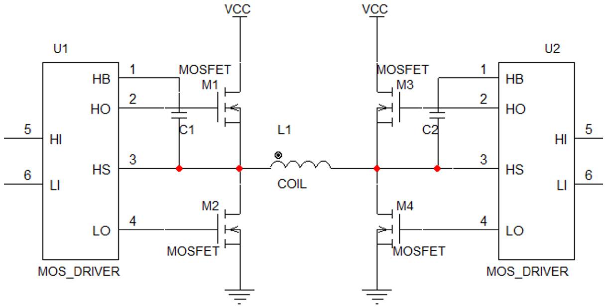
To address these drawbacks of conventional power amplifiers, switch-mode power amplifiers, particularly Class-D types, are gaining popularity. In a Class-D power amplifier, the output transistors operate as electronic switches, alternating between fully ON and fully OFF states at high frequency. This switching minimizes switching and conduction power losses, resulting in remarkably high amplifier efficiency [15, 16]. Figure 3 illustrates the circuit diagram of a full-bridge (H-bridge) Class-D amplifier, a configuration widely used in modern high-efficiency designs. The combination of a Class-D power amplifier with multi-frequency selective harmonic elimination pulse-width modulation (SHE-PWM) enables direct generation of complex multi-frequency current signals from a direct current (DC) power source, without requiring linear amplification of each frequency component. This approach overcomes the efficiency bottleneck of conventional amplifiers while maintaining high spectral purity of the output current signals and their harmonics. It allows real-time generation of broadband excitation signals with both high efficiency and high spectral purity, making it suitable for advanced multi-frequency eddy-current detection systems. Table 1 summarizes the performance differences between Class-D and Class-AB power amplifiers.

4.1 Fourier series representation of inductor current
To achieve high SNR, low drift, and repeatability in eddy-current–based localization of metallic foreign bodies in the human body, the transmitter must not only provide sufficient excitation strength but also deliver a controllable and stable excitation spectrum. This requirement is particularly critical under synchronous multi-frequency excitation, where inter-frequency amplitude and phase consistency directly determines the stability of I/Q-demodulated features and the achievable localization accuracy. Although Class-D power amplifiers offer high efficiency and are suitable for portable implementations, their switching outputs inherently contain rich harmonic components. If such harmonics are not properly controlled, the tissue–coil system may exhibit additional background responses, baseline drift, and inter-frequency crosstalk, thereby reducing detectability of tiny targets and increasing the risk of false positives. To address this issue, this study adopts a SHE strategy, optimizing switching angles to synthesize the desired excitation at target frequencies while suppressing critical non-target harmonics. This approach enhances the robustness of multi-frequency detection and improves the reliability of target localization.
In the SHE strategy, the switching angles are designed to constrain the output harmonic spectrum. As a result, the excitation current achieves the desired amplitude at the designated target frequencies while minimizing specific non-target harmonic components.
The periodic pulse-width modulation (PWM) voltage generated by the power electronic converter can be represented using a Fourier series, which forms the basis for harmonic angle optimization, as shown in Equation (1) [17]:

where a0 indicates the DC term, an the cosine coefficients, and bn the sine coefficients. The Fourier series representation of the PWM waveform is inherently complex due to multiple switching intervals and asymmetric pulse durations.
To cosine the analytical solution and facilitate harmonic management, the PWM waveforms can be assumed to possess quarter-wave symmetry. Under this assumption, the waveform exhibits half-period sign inversion symmetry, which mathematically eliminates certain Fourier components, specifically the DC term, even harmonics, and sine coefficients of odd harmonics. This assumption greatly simplifies the nonlinear equations used to determine the switching angles for the SHE-PWM strategy, enabling effective synthesis of the multi-frequency excitation waveform.
In the full-bridge Class-D power amplifier under the symmetrical conditions, the voltage waveform applied to the load can be described in a compact Fourier series form. The resulting series, presented in Equation (2), provides the mathematical basis for determining the targeted harmonic components and their corresponding switching angles in the SHE-PWM approach:

Under the quarter-wave symmetry assumption, the cosine Fourier coefficients related to the harmonic components of the output voltage can be further derived. These coefficients quantify the amplitudes of the retained harmonics and relate the desired output spectrum to the switching angles of the inverter. The general form of the cosine series coefficients is expressed in Equation (3):

Here, n takes only odd integers due to the use of quarter-wave symmetry, which restricts harmonics to odd orders. αi denotes the switching angles of the PWM waveform, i.e., the time at which the output voltage transitions between levels within a half-wave cycle. V0 represents the drain voltage of the MOSFET switch, which, in the context of the full-bridge Class-D amplifier represented in Figure 2, corresponds to the supply voltage VCC.
In the above Class-D power amplifier system investigated in this study, the excitation coil can be approximated as an ideal inductive load. By this approach, the terminal voltage and current satisfy the constitutive relation of an ideal inductor, which facilitates waveform synthesis. In this case, the instantaneous voltage across the coil is given by:

where L denotes the inductance of the excitation coil. Therefore, the instantaneous current through the excitation coil can be modeled as the time integral of the applied pulsed voltage:

This model captures the accumulative property of the inductor current, reflecting the increase in magnetic energy of the coil as a function of the applied voltage and duration of the excitation signal. The output voltage of the Class-D power amplifier takes only discrete values, usually +V0 and -V0, forming a series of rectangular pulses in the time domain. Accordingly, the current through the inductive load represents the integral of these voltage pulses. Figure 4 illustrates the voltage waveform and the corresponding current waveform.
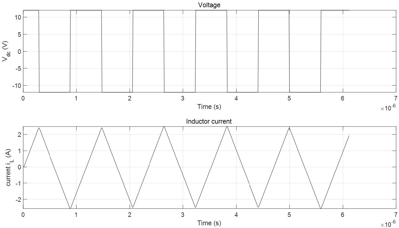
Let ω=2π/T denote the basic angular frequency of the periodic excitation signal. By substituting Equations (2), (3), and (5) into the previous expressions, the instantaneous current in the excitation coil can be represented as a Fourier series expansion, as in Equation (6). The coefficients bn, representing the amplitude of the harmonic components in the coil current, are described in Equation (7).


4.2 Frequency selection of inductor current
In the previous section, the Fourier series representation of the inductor current was derived from the PWM voltage waveform of the inverter. Consequently, various current waveforms can be synthesized by appropriately selecting the cosine series coefficients bn. In this case, the proper selection of these coefficients is critical for defining the quality and spectral content of the excitation currents.
To obtain a physically realizable and spectrally controlled current shape, the desired shape must first be defined in the time domain. Morphologically, each switching interval should exhibit a high level of linearity to allow an accurate approximation using piecewise linear segments. In addition, to simplify the Fourier series coefficients and maintain a manageable mathematical form, the target waveform is designed with quarter-wave symmetry, consisting of the fundamental and odd harmonics. This design preserves symmetry across each half cycle, eliminates redundant even-order harmonics, while retaining only the harmonic components required for multi-frequency excitation.
In eddy-current-based assistance for localization of metallic foreign bodies within the human body, multi-frequency excitation is commonly employed to obtain complementary electromagnetic response features, so as to accommodate variations in both target materials (ferromagnetic and non-ferromagnetic) and burial depth or orientation. The theoretical basis is that the eddy-current distribution and associated secondary magnetic field are jointly determined by the electrical conductivity σ, magnetic permeability μ, and the excitation angular frequency ω, exhibiting pronounced frequency dependence. According to the skin effect, the characteristic skin depth is given by:

As the excitation frequency increases, the skin depth decreases: high-frequency excitation concentrates eddy currents near the target surface, thereby enhancing sensitivity to superficial and small-sized foreign bodies; in contrast, low-frequency excitation provides a greater effective electromagnetic penetration depth, thereby improving detectability of deeply embedded targets. Moreover, materials with higher 𝜇 and 𝜎 (e.g., ferromagnetic metals or high-conductivity metals) tend to exhibit stronger skin effects and more pronounced amplitude/phase variations at the same frequency, facilitating material discrimination and localization.
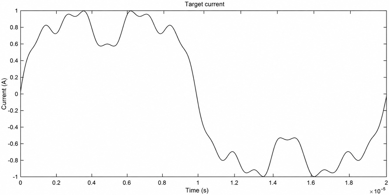
Based on this principle and leveraging the spectrally controllable synthesis enabled by SHE, this study selects 50 kHz, 150 kHz, 350 kHz, and 850 kHz as the multi-frequency excitation tones. The corresponding current waveform are designed to provide complementary amplitude–phase responses for subsequent signal processing. By using synchronous multi-frequency excitation, an amplitude–phase (I/Q) feature space can be constructed, allowing joint evaluation of responses across frequencies. This approach improves robustness against tissue-background effects, variations in electromagnetic coupling, and motion-induced amplitude/phase perturbations, thereby enhancing both the detectability and localization resolution for tiny metallic foreign bodies in the human body. The mathematical expression of the synthesized inductor current can is given by Equation (9), and the corresponding time-domain current waveforms are illustrated in Figure 5.

4.3 Optimization of the spectral coefficients of inductor current
The primary objective of the SHE-PWM is to modulate the low-order harmonics of the output waveform through optimized switching angles αi. This approach allows elimination of unwanted harmonics from high-power converters while preserving the required spectral characteristics of the excitation signal. A major challenge in implementing SHE-PWM lies in solving a system of nonlinear transcendental equations that map the switching angles αi to the amplitudes of the harmonics. The complexity of this system depends on the waveform characteristics and the number of discrete voltage levels involved.
Several methods have been proposed to address this challenge, including numerical solutions, resultant theory methods, and optimization-based techniques. Numerical methods usually face difficulties due to the nonlinear expressions inherent in standard SHE-PWM models, especially when high-order harmonics or two-level inverter topologies are used. Resultant theory approaches encounter increasing computational complexity as the polynomial order rises with the number of harmonics to be eliminated.
With advances in computational power, optimization-based strategies have become the preferred approach. In this framework, the SHE-PWM equations are reformulated as an optimization problem subject to constraints. The objective function is defined as the residual magnitude of the undesired harmonics, with the goal of minimizing this value. Constraints enforce the elimination of targeted harmonics and the symmetry of the waveform.
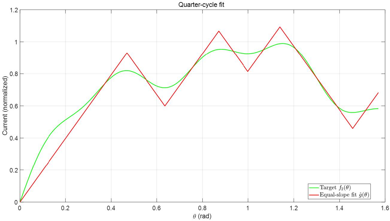
In this context, the switching angles αi can be determined via an optimization algorithm. The procedure begins by identifying the local extrema of the target current waveform. These extrema serve as initial estimates for the switching angles, providing a valid starting point for subsequent iterations. In system employing a single H-bridge configuration, the slope of the inductor current remains constant in magnitude during each switching interval, allowing the previous target current waveform to be approximated by line segments with equal slope magnitude.
Figure 6 illustrates the optimization procedure for one-quarter of the waveform duration (θ=π/2≈1.57). The green curve represents the desired target current in the first quarter of the waveform, while the red polylines show piecewise-linear approximation used in the optimization. The remaining three quarters of the waveform are derived through symmetry. The initial switching angles derived from this approximation method are provided in Table 2.

However, when a suitable initial guess for the switching angles exists, gradient-based algorithms can converge substantially faster than stochastic or population-based algorithms [18]. In this study, a gradient-based algorithm was used to determine the amplitudes of the harmonic components, as formulated in Equation (10):

Here, the modulation index is defined as:

where Vp represents the amplitude of the pth harmonic of the output voltage, and V0 denotes the DC bus voltage of the Class-D amplifier. The weighting factor μp scales the contribution of each harmonic to the objective function. Φ indicates the set of desired harmonics to be accurately synthesized, while Ψ represents the set of undesired harmonics to be reduced. The parameter εp defines the permissible level of each non-target harmonic, acting as a soft constraint to prevent excessive distortion.
Minimizing the residual error between the calculated Fourier coefficient bp and the modulation index mp, while respecting the constraints on non-target harmonics, enables iterative refinement of the switching angles to accurately reproduce the desired harmonics and suppress undesired components.
Using the initial switching angles derived from the piecewise-linear approximation of the target current waveform g(θ) and the coefficient definition from Equation (7), the harmonic components can be analytically derived by Equation (12):

At each switching angle αi, two successive voltage transitions occur: from +V0 to 0 and then from 0 to −V0, or vice versa depending on the switch polarity, which must be accounted for in the Fourier series computation.
When θ=π/2, only a single downward transition (+V0 to 0) occurs, corresponding to the end of quarter cycle. Substituting Equation (12) into the residual minimization problem of Equation (10) yields Equation (13), which explicitly relates the residual harmonic amplitudes to the switching angles, enabling selective synthesis of harmonics in the Class-D power amplifier system.

The initial parameters for the optimization algorithm are shown in the first column of Table 3. In this case, the weighting factors μp were set to unity (μp=1). Once the initial switching angles and weights are determined, the constrained optimization problem is solved using the fmincon function in MATLAB. The objective function quantifies the deviation between predicted and target harmonic magnitudes, while the constraints enforce the permissible bounds for non-target harmonics.

The fmincon function (constrained function minimization) is the primary procedure within the MATLAB Optimization Toolbox used to solve constrained continuous optimization problems where the objective and constraint functions are continuously differentiable. This function can handle continuous decision-variable problems subject to linear and/or nonlinear constraints. Figure 7 illustrates the optimization results for the switching angles as formulated in Equation (12).
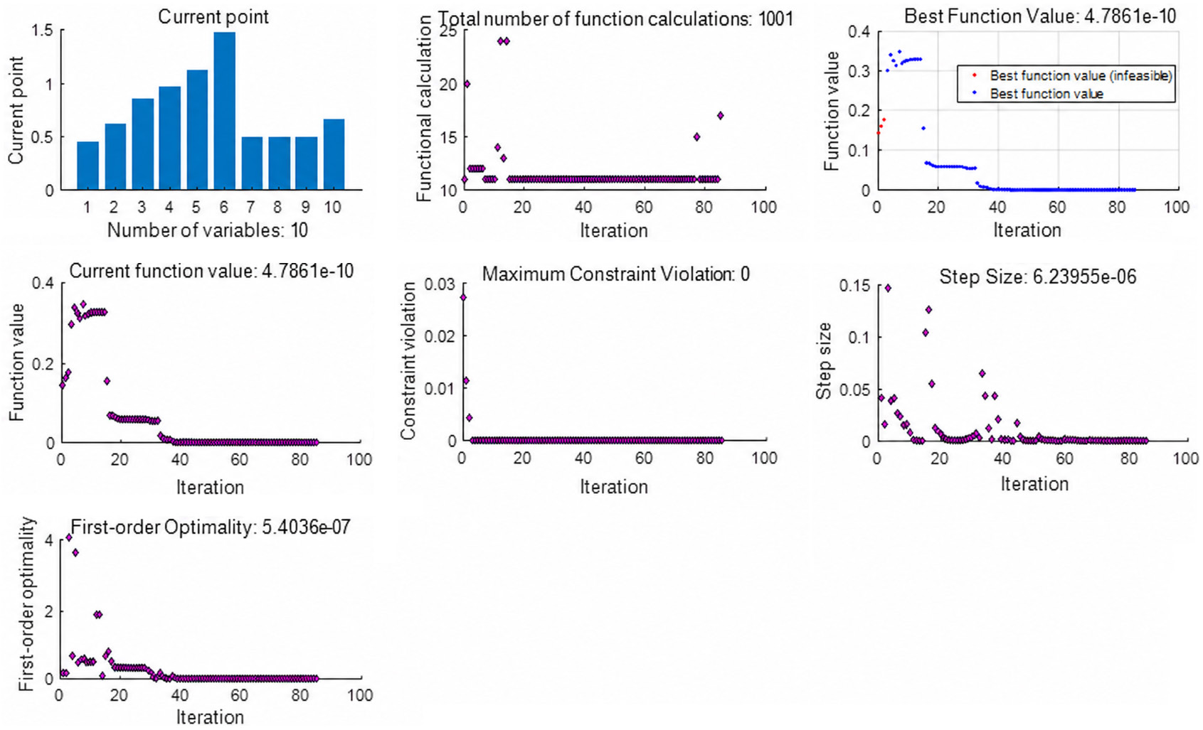
The Maximum Constraint Violation metric decreases drastically from approximately 3×10⁻² in the early iterations to nearly zero by the 10–15th iteration. This trend indicates that the barrier term and line-search procedures within the interior-point method effectively guide the iterates from infeasible to feasible regions. Once feasibility is achieved, the iterates remain strictly feasible throughout the rest of the optimization procedure, demonstrating that all constraints are satisfied.
Simultaneously, the Best Function Value decreases steadily from approximately 3.5×10⁻¹ to the order of 10-4 over 30-40 iterations, eventually stabilizing at a minimal of 4.7861×10⁻¹⁰. The convergence behavior can be understood by examining the plots of feasible and infeasible solutions. In the initial iterations, several infeasible points (red stars in Figure 7) approach the feasible region but remain constrained by the limits. However, the best feasible objective (blue stars) steadily improves until it converges to the best infeasible objective at the global minima point. This observation clarifies a common misconception that the best feasible point must be optimized before the infeasible solution. Ultimately, the evolution of the Best Function Value reflects the transition from satisfying the feasibility constraints to the final optimization of the switching angles within the feasible region, thereby minimizing the residuals of the harmonic components.
The Step Size parameter displays several backtracking and enlargement pulses during the first TEN iterations. After this phase, the step size stabilizes at approximately 10-4, indicating the onset of the local refinement phase of the optimization. This pattern of behavior is consistent with the Interior-Point Algorithm’s barrier parameter update and centralization mechanism, wherein the solver fine-tunes the solution in the region of the optimal point once feasibility has been established.
The First-Order Optimality value reduces from an initial order of O(1) to approximately 5.4×10⁻⁷, remaining below the default optimality tolerance of approximately 10-6 used in the fmincon solver. Along with the step size reduction and stabilization of the objective function, these results indicate that the algorithm has approached a stationary point satisfying the Karush-Kuhn-Tucker (KKT) conditions, where the first-order necessary conditions for constrained optimality are approximately satisfied.
The number of function evaluations was 1,001, requiring fewer than 100 iterations. In the case of a ten-dimensional optimization problem with six switching angles and four modulation indices involving nonlinear equality and inequality constraints, this moderate computational effort reflects good differentiability of the objective and constraint functions along with minimal backtracking during the line search.
The current point bar chart shows that the six optimized switching angles converge to the range of 0.5–1.5 radians, remaining strictly within their prescribed bounds (0 to π/2). This implies that the solution is largely driven by harmonic constraints rather than boundary saturation. Similarly, the four modulation indices converge to the range of 0.5–0.8, well within he physically acceptable limits. Together with the observation that the Maximum Constraint Violation remains at zero, this confirms feasibility and realizability of the solution.
In general, the optimization algorithm exhibits the conventional behavior of an interior-point method: (1) rapid approach toward feasibility, (2) orderly and monotonic decrease of the objective function, (3) gradual reduction of the step size accompanied by improved first-order optimality, and (4) attainment of a strictly feasible solution satisfying the KKT conditions approximated to the desired precision. The final objective function value of 4.7861×10⁻¹⁰ suggests that the residual harmonics are minimized to numerical precision, confirming accurate representation of both target and non-target harmonics within the prescribed thresholds.
From an engineering perspective, the optimized switching angles and modulation indices jointly achieve the desired spectral characteristics without boundary saturation, ensuring robust tolerance to timing errors and dead-time quantization. Figure 8 compares the voltage-current waveforms before and after optimization. The reduction in harmonic distortion validates the effectiveness of the proposed method in generating high-purity multi-frequency excitation currents suitable for high-sensitivity localization of tiny metallic foreign bodies in the human body.
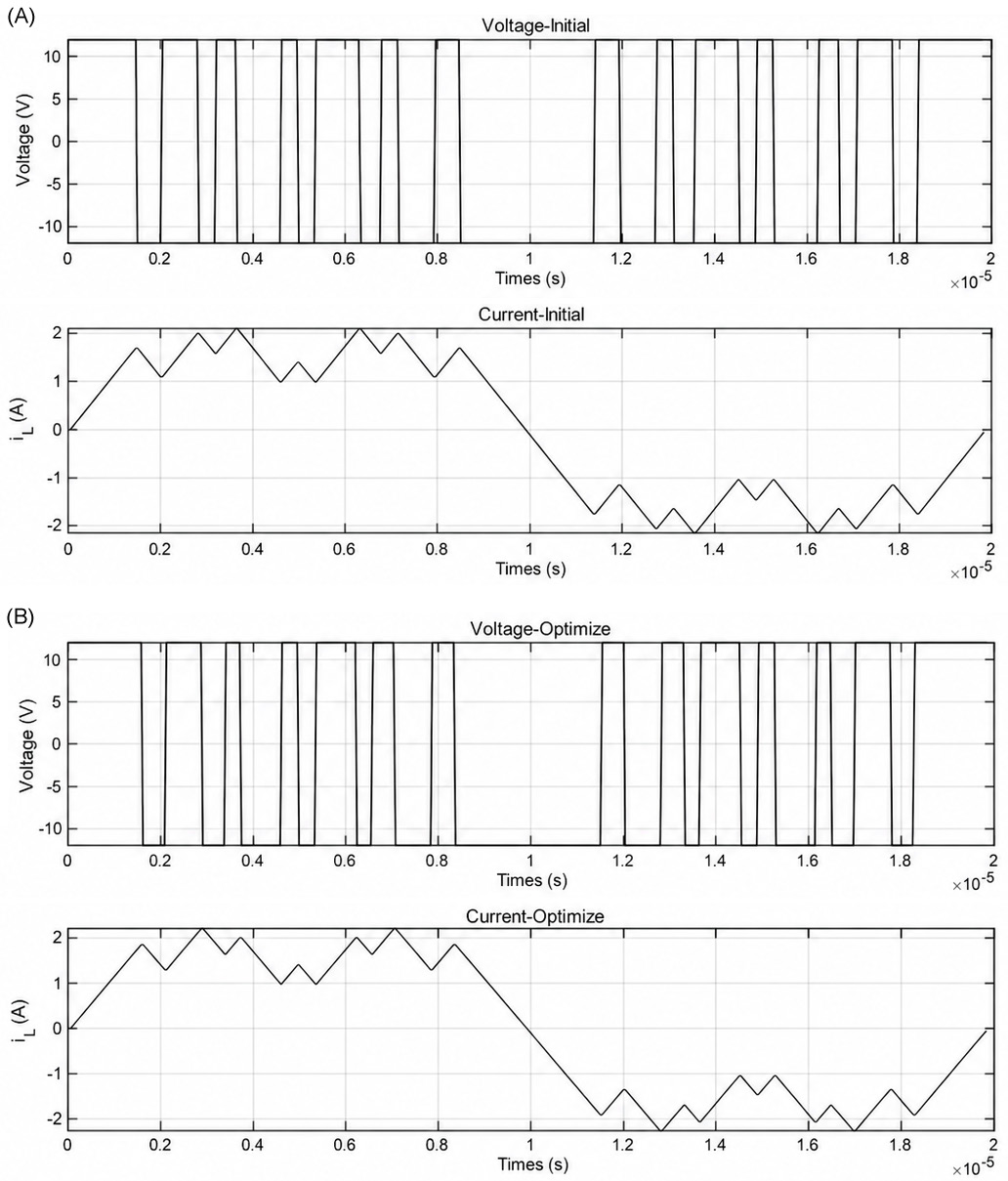
Figure 8. Initial and optimized voltage-current waveforms of the excitation coil. (A) Initial voltage-current waveforms prior to SHE-PWM optimization; (B) Voltage-current waveforms after optimization, showing improved harmonic purity and adherence to the target multi-frequency excitation profile.
5.1 Device selection
As illustrated in Figure 8, the output voltage waveform exhibits a maximum switching frequency of approximately 3–4 MHz. Accordingly, the gate driver and MOSFET devices must operate reliably at such high switching speeds. In this study, the isolated gate driver IC 2EDF7275K was employed to drive the power stage. This gate driver provides galvanic isolation between the power and control circuits, mitigating the propagation of high-current transients from the power stage to sensitive control inputs, such as those of the FPGA, which could otherwise lead to permanent damage. The 2EDF7275K IC supports switching frequencies of up to 10 MHz, easily accommodating the PWM switching pulses described previously. Moreover, it allows flexible gate-level adjustments, facilitating circuit tuning and debugging.
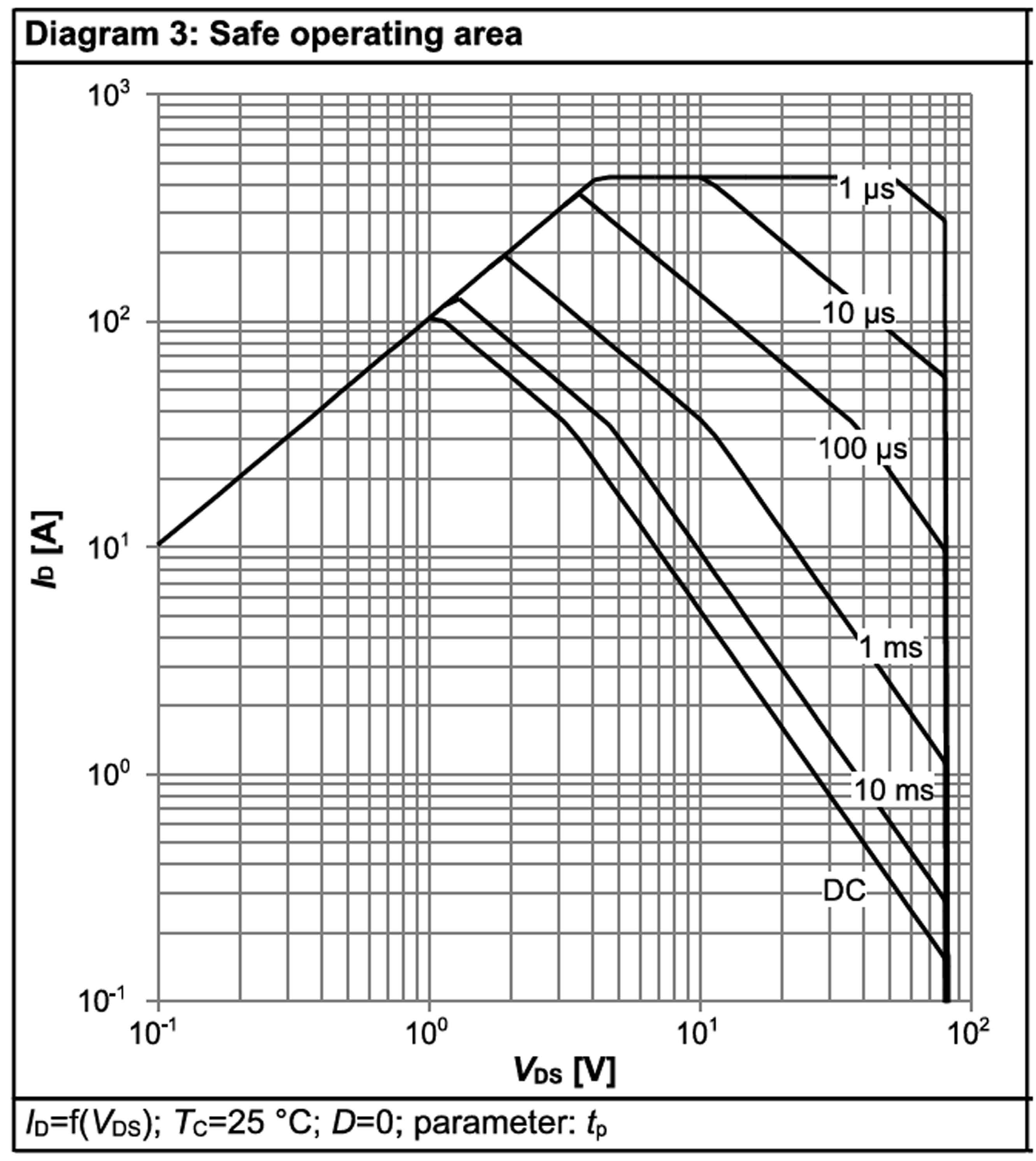
For the power switching components, BSC057N08NS3 MOSFETs were chosen. These devices have a drain-source voltage of 80 V, a typical on-resistance RDS(on) of 5.7 mΩ, along with fast transition times (tr≈14 ns, tf≈9 ns), minimizing transition losses and reducing waveform distortion during high-frequency Class-D operation. According to the Safe Operating Area (SOA) diagram shown in Figure 9, the MOSFETs can be safely operated under the chosen conditions of 12 V input and a 2 A drain current. These specifications provide sufficient margin to ensure reliable performance during continuous high-frequency switching, enabling stable excitation currents in the coil necessary for high-sensitivity eddy-current detection of tiny metallic foreign bodies.
5.2 Hardware circuit simulation
Figure 10 shows the voltage and current waveforms and their corresponding spectra, obtained through PSpice simulations. PSpice is a widely used general-purpose circuit simulator in the field of electronic design automation (EDA), mainly used to evaluate and develop analog and mixed-signal (analog-digital) electronic circuits. It allows designers to predict circuit performance before physical implementation.
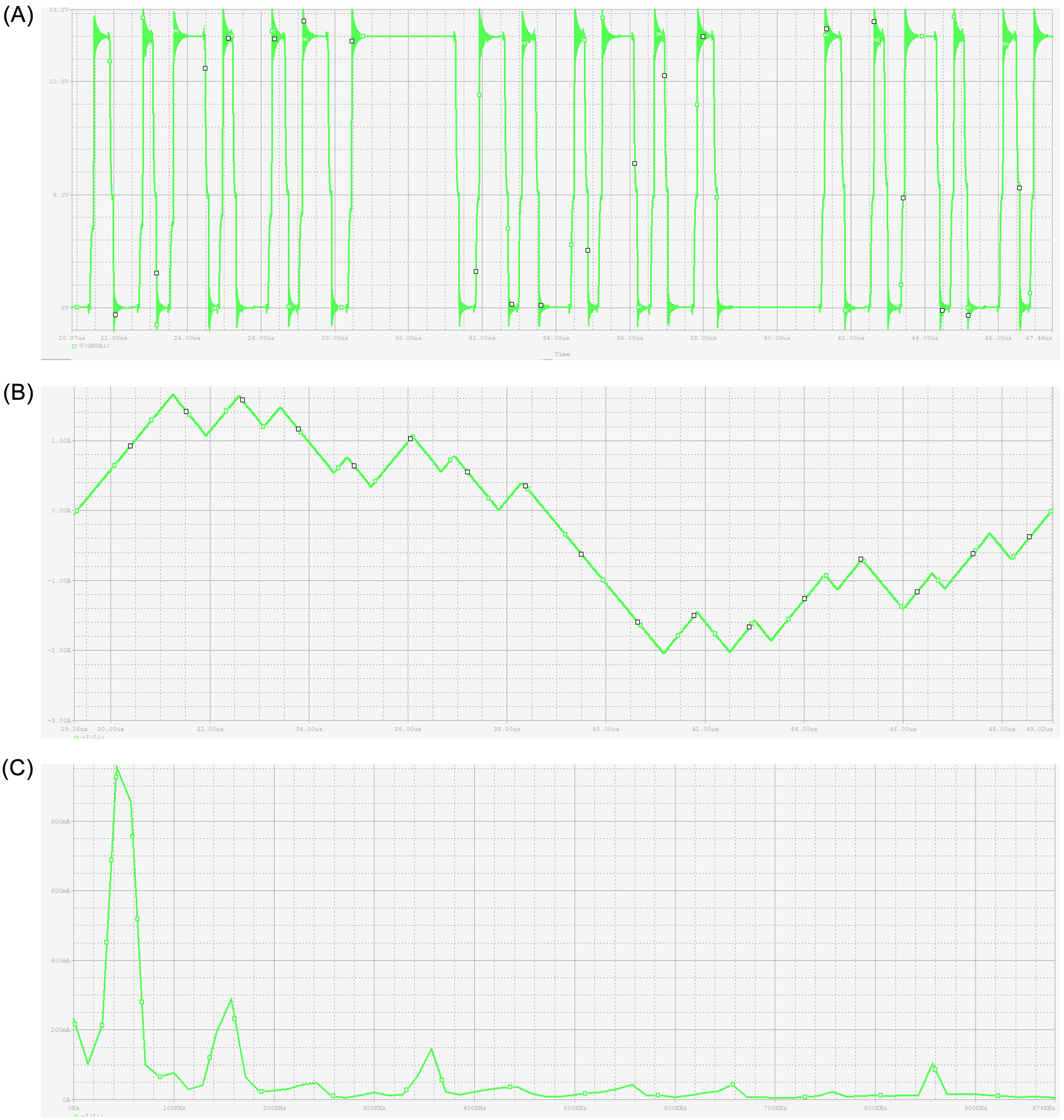
Figure 10. Voltage, current, and current spectrum of the excitation coil from hardware circuit simulation. (A) Time-domain voltage waveform of the H-bridge output; (B) Time-domain current waveform through the excitation coil; (C) Frequency-domain spectrum of the coil current showing multi-frequency excitation peaks at 50 kHz, 150 kHz, 350 kHz, and 850 kHz.
Simulation outcomes indicate slight oscillations in the output voltage waveform during switching transitions. These slight oscillations, however, do not affect circuit functionality. In the time-domain current waveform of the excitation coil, the inductor current closely follows the target waveform, confirming the correct operation of the Class-D power amplifier and the effectiveness of the SHE-PWM control strategy.
Frequency-domain analysis further confirms these observations. Distinct spectral peaks appear at 50 kHz, 150 kHz, 350 kHz, and 850 kHz, accurately matching the four predefined excitation frequencies. Simultaneously, the amplitudes of non-target harmonics remain below the specified thresholds, indicating that the optimized switching angles and modulation indices successfully achieve precise harmonic synthesis. These results confirm that the excitation current exhibits a well-defined multi-frequency pattern with high spectral purity, which is essential for robust and accurate eddy-current detection of tiny metallic foreign bodies in the human body.
5.3 Hardware circuit design
The power supply module of the hardware platform is designed to provide multiple regulated voltage rails to satisfy the requirements of various circuit sub-components. As illustrated in Figure 11, the initial 12 V DC input is first stepped down to 8 V to provide the gate-drive voltage for the MOSFETs in the H-bridge power stage. To ensure galvanic isolation between the control and power planes, the 8 V line follows is further stepped down using an isolated DC-DC converter to provide 5 V for the gate-driver ICs. Subsequently, a linear voltage regulator generates the 3.3–5 V control-side voltages needed by the driver circuitry.
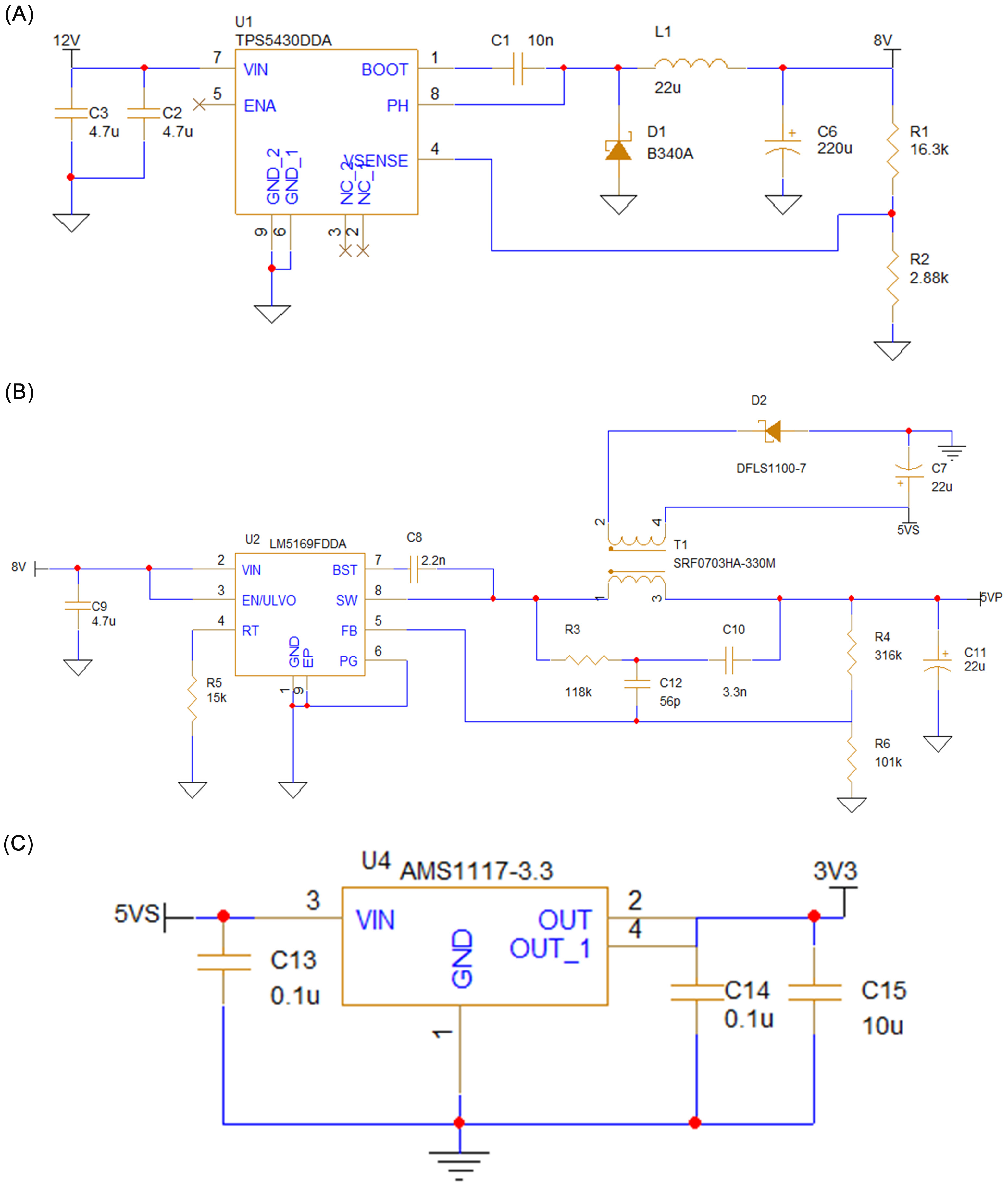
Figure 11. Power supply module of the hardware platform. (A) Step-down conversion from 12 V to 8 V; (B) Isolated DC-DC conversion from 8 V to 5 V; (C) Linear regulation from 5 V to 3.3 V.
Figure 12 illustrates the schematic diagram of the H-bridge module. For clarity, only half of the bridge is illustrated, as the other half is symmetrical. The COL+ node connects to the first terminal of the excitation coil, while the second terminal is connected to COL−. The input network pins IN+ and IN− (pins 3 and 2 of the second 2EDF7275K isolated gate-driver IC) are configured to guarantee complementary switching between the two half-bridges and to maintain the desired differential phase relationship of the output voltage.
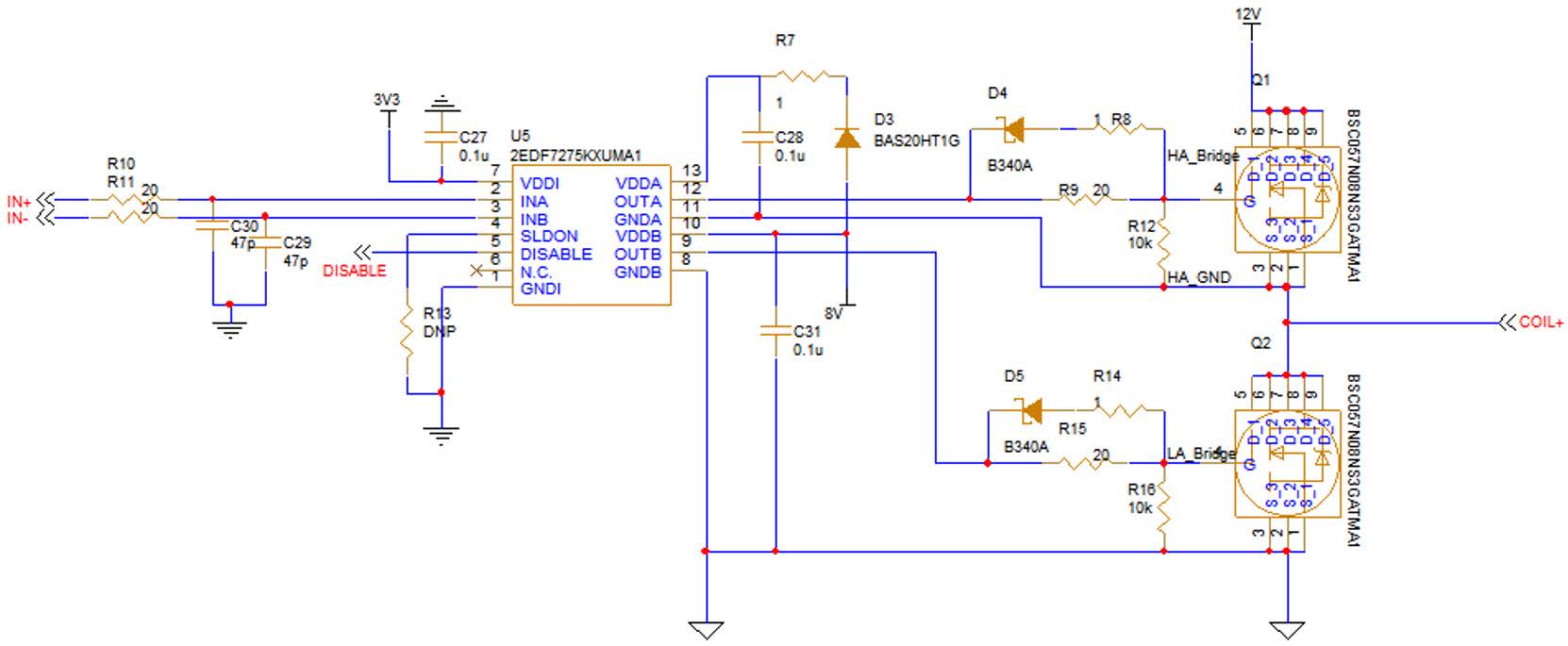
In the gate-drive circuitry, B340A Schottky Rectangular Diodes (D4 & D5) are paralleled with resistors R9 & R13. This configuration facilitates rapid turn-off transitions of the MOSFETs, as the current is directed through the low-impedance path of the B340A Rectangular Diodes, reducing gate-charge removal time [19-21]. During turn-on, the gate charge current flows from the driver’s output (OUTA and/or OUTB) to the MOSFET gate. In this phase, the B340A diodes are reverse-biased and non-conductive, and the resistive network controls the gate charging rate, resulting in a “slow turn-on, fast turn-off” behavior. This asymmetrical switching mitigates parasitic inductance-induced voltage overshoot and ringing while maintaining efficient switching transitions and minimizing electromagnetic interference in the H-bridge circuit.
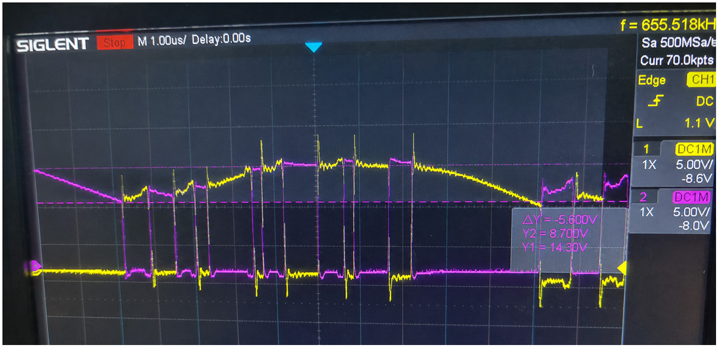
Figure 13 illustrates the experimentally recorded H-bridge output voltage. In this diagram, the yellow curve corresponds to the voltage at the COL+ terminal of the excitation coil, whereas the pink curve corresponds to the COL− terminal. A clear voltage sag appears across the coil during specific intervals, attributed to the charge-discharge behavior of the bootstrap capacitor (C24) used in the gate-drive circuit of the high-side MOSFETs. When the low-side MOSFET conducts for a short duration, the bootstrap capacitor is not fully charged. Consequently, during the subsequent long conduction interval of the high-side MOSFET, the capacitor discharges over an extended period, resulting in reduced gate-drive voltage and the observed voltage sag across the coil.
This study addresses the clinical challenge of assisted screening and localization of tiny metallic foreign bodies in the human body (e.g., suture needles, hemostatic clips, and shrapnel). Leveraging the SHE approach, we developed a transmitter driving scheme capable of generating synchronous multi-frequency excitation currents, providing an energy-efficient and spectrally controllable excitation-circuit foundation for eddy-current-based detection systems.
By optimizing the switching angles, the transmitter achieves precise current components at the designated target frequencies while effectively suppressing critical non-target harmonics. This, in turn, mitigates unwanted background responses, baseline drift, and inter-frequency crosstalk in the tissue–coil coupling system, thereby improving the stability and repeatability of multi-frequency excitation. Furthermore, circuit-level simulations and hardware implementation validate the engineering feasibility of the proposed scheme. These results provide a robust hardware foundation for future development of clinical-oriented multi-frequency eddy-current detection techniques, enabling feature-based discrimination and accurate localization of tiny metallic foreign bodies.
Author contributions
Yuming Liu performed data acquisition, processing, analysis and model building and wrote the manuscript. Piding Li made substantial contributions to data analysis and manuscript preparation.
Funding
This research received no external funding.
Data availability
This study utilized only publicly available datasets.
Ethics approval and consent to participate
Not applicable.
Consent for publication
We agree to the publication of this manuscript in both print and electronic formats in ZENTIME, and grant the publisher permission to make necessary editorial and formatting revisions to the manuscript.
Competing interests
The authors declare that they have no competing interests.
Acknowledgements
Not applicable.
[1] Bozorgmehr R, Bahadorinia M, Pouyanfar S, Ahmadinejad M, Bahri MH, Bagherpour JZ. A rare case of abdominal foreign bodies; laparoscopic removal of a sewing needle. Ann Med Surg (Lond). 2022 Oct;82:104747. https://doi.org/10.1016/j.amsu.2022.104747
[2] Hall Barbosa C. Localization of firearm projectiles in the human body using a superconducting quantum interference device magnetometer: A theoretical study. Rev Sci Instrum. 2004 Jun 1;75(6):2098-2106. https://doi.org/10.1063/1.1753679
[3] AbdAlla AN, Faraj MA, Samsuri F, Rifai D, Ali K, Al-Douri Y. Challenges in improving the performance of eddy current testing: Review. Meas Control. 2019 Jan;52(1-2):46-64. https://doi.org/10.1177/0020294018801382
[4] Grochowalski JM, Chady T. Rapid identification of material defects based on pulsed multifrequency eddy current testing and the k-nearest neighbor method. Materials. 2023 Oct 11;16(20):6650. https://doi.org/10.3390/ma16206650
[5] Svatos J, Vedral J, Pospisil T. Advanced instrumentation for polyharmonic metal detectors. IEEE Trans Magn. 2016 May;52(5):1-4. https://doi.org/10.1109/TMAG.2015.2507780
[6] Yamazaki S, Nakane H, Tanaka A. Basic analysis of a metal detector. IEEE Trans Instrum Meas. 2002 Aug;51(4):810-814. https://doi.org/10.1109/TIM.2002.803397
[7] Hu W, Liu Z. Study of metal detection based on chaotic theory. In: 2010 8th World Congress on Intelligent Control and Automation; 2010 Jul 7-9; Jinan, China. IEEE; 2010. p 2309-2314. https://doi.org/10.1109/WCICA.2010.5554170
[8] Garcia-Martin J, Gomez-Gil J, Vazquez-Sanchez E. Nondestructive techniques based on eddy current testing. Sensors. 2011;11(3):2525-2565. https://doi.org/10.3390/s110302525
[9] Bernieri A, Betta G, Ferrigno L, Laracca M. Crack depth estimation by using a multi-frequency ECT method. IEEE Trans Instrum Meas. 2023 Mar;62(3):544-552. https://doi.org/10.1109/TIM.2012.2232471
[10] Machado MA. Eddy currents probe design for NDT applications: A review. Sensors. 2024 Sep 7;24(17):5819. https://doi.org/10.3390/s24175819
[11] Sophian A, Tian G, Fan M. Pulsed eddy current non-destructive testing and evaluation: A review. Chin J Mech Eng. 2017 May;30:500-514. https://doi.org/10.1007/s10033-017-0122-4
[12] Blitz J, Peat TS. The application of multi-frequency eddy currents to testing ferromagnetic metals. NDT E Int. 1981 Feb;4(1):15-17. https://doi.org/10.1016/0308-9126(81)90058-4
[13] Antoun CA, Wursch C, Kochli C, Perriard Y. Balanced metal detector based on optimized frequencies and spatial phase profile responses to differentiate metal rods. IEEE Magn Lett. 2017;8:1-5. https://doi.org/10.1109/LMAG.2017.2674619
[14] Zhang B, Yin G, Zhang Y, Lin J. Research on highly sensitive electromagnetic method based on balance coil for underground metal detection. IOP Conf Ser: Earth Environ Sci. 2021;660(1):012004. https://doi.org/10.1088/1755-1315/660/1/012004
[15] Duraij M, Xiao Y, Zsurszan G, Zhang Z. A comparative study on Class AB and Class D amplifier topologies for high temperature power line communication circuits. In: 2021 IEEE International Symposium on Power Line Communications and its Applications (ISPLC); 2021 Oct 26-27; Aachen, Germany. IEEE; 2021. p. 102-107. https://doi.org/10.1109/ISPLC52837.2021.9628537
[16] Mei S, Hu Y, Xu H, Wen H. The class D audio power amplifier: A review. Electronics. 2022 Oct 9;11(19):3244. https://doi.org/10.3390/electronics11193244
[17] Dahidah MSA, Konstantinou G, Agelidis VG. A review of multilevel selective harmonic elimination PWM: Formulations, solving algorithms, implementation and applications. IEEE Trans Power Electron. 2015 Aug;30(8):4091-4106. https://doi.org/10.1109/TPEL.2014.2355226
[18] Boyd S, Vandenberghe L. Convex optimization. Cambridge (UK): Cambridge University Press; 2004. 727 p. https://doi.org/10.1017/CBO9780511804441
[19] Rujas A, López VM, Mir L, Nieva T. Gate driver for high power SiC modules: Design considerations, development and experimental validation. IET Power Electron. 2018;11(6):977-983. https://doi.org/10.1049/iet-pel.2017.0535
[20] Jiang Y, Feng C, Yang Z, Zhao X, Li H. A new active gate driver for MOSFET to suppress turn-off spike and oscillation. Chin J Electr Eng. 2018 Jun;4(2):43-48. https://doi.org/10.23919/CJEE.2018.8409349
[21] Aboadla EH, Khan S, Abdul Kadir K, Md Yusof Z, Hababci MH, Habib S, et al. Suppressing voltage spikes of MOSFET in H-bridge inverter circuit. Electronics. 2021 Feb 5;10(4):390. https://doi.org/10.3390/electronics10040390
ISSN: 2957-5478
Volume 4, Issue 2
June 2026
Pages: 77-177


 Log In

 On This Page
 CITE
CITE