An influenza forecasting model based on RG-EEMD-TFT

Keywords: Influenza forecasting, Influenza-like illness, Ensemble empirical mode decomposition, Reconstruction grouping, Time series forecasting, Temporal fusion transformer

Influenza is an acute respiratory infectious disease with marked seasonal characteristics and remains a major threat to public health. Accurate forecasting of influenza activity is essential for improving the allocation of healthcare resources and supporting evidence-based epidemic control measures. Seasonal influenza imposes a substantial burden through hospitalizations and mortality, and its timing, intensity, and spatial distribution vary considerably, creating uncertainty and pressure on healthcare systems. Early prediction of influenza activity enables public health authorities to anticipate epidemic patterns over the coming weeks or months and to make timely decisions regarding antiviral distribution, vaccination, staffing, bed allocation, and community-level interventions [1]. In recent years, considerable attention has been directed toward the development of deep learning methods for influenza forecasting [2,3].

Despite these advances, important challenges remain in modeling complex temporal patterns and effectively integrating information from multiple sources. Influenza surveillance data are inherently nonlinear, non-stationary, and multi-scale, containing long-term trends, periodic fluctuations, and stochastic disturbances [4]. As a result, raw influenza time series often exhibit strongly entangled patterns across multiple time scales, making it difficult to separate trend-related signals from high-frequency noise and to model non-stationary sequences effectively. Traditional recurrent neural networks (RNNs) and their variants, including long short-term memory networks (LSTMs), typically encode multivariate time series through simple concatenation or uniform feature representation. Such approaches often fail to capture dynamic correlations and heterogeneous temporal variation across features. This limitation arises from the lack of explicit modeling of inter-variable relationships, which hinders the modeling of complex temporal dynamics and reduces both interpretability and predictive accuracy [5].

To address these limitations, this study proposes a forecasting framework that integrates ensemble empirical mode decomposition (EEMD), reconstruction grouping (RG), and a Temporal Fusion Transformer (TFT). Experiments on real-world influenza surveillance data show that the proposed RG-EEMD-TFT framework outperforms several baseline approaches in both accuracy and stability, highlighting the value of adaptive decomposition, feature reconstruction, and transformer-based temporal modeling for complex public health time series.

2.1 Principle of ensemble empirical mode decomposition (EEMD)

Ensemble Empirical Mode Decomposition (EEMD) is an improved data processing method developed from Empirical Mode Decomposition (EMD), in which normally distributed random white noise is added to the signal. Particularly, the procedure repeatedly introduces white noise into the original signal and EMD decomposition is conducted, with the findings being averaged. This procedure effectively alleviates the mode mixing problem inherent in the traditional EMD method, thereby improving the stability and reliability of the decomposition results [6]. Compared with EMD, EEMD can adaptively perform multi-scale decomposition of complex time series, avoiding excessive decomposition and mode mixing. Consequently, it is more suitable for processing nonlinear and non-stationary signals [7]. The specific procedure is described as follows:

First, the normally distributed random white noise m_i(t) is added to the original time series y(t) to construct a new time series:

where y(t) denotes the original time series data, m_i(t) represents the normally distributed random white noise signal, and y_i(t)denotes the time series obtained after the i-th addition of white noise.

Next, the EMD algorithm is applied to the updated time series to extract the corresponding intrinsic mode functions D_i,j(t) and the residual term x_i(t):

where D_i,j(t)denotes the j-th intrinsic mode function (IMF) obtained after the i-th addition of white noise, x_i(t) represents the residual term, and N denotes the number of IMF components.

Finally, the n groups of D_i,j(t) and x_i(t) are averaged to obtain the final decomposition results H_j(t) and R(t):

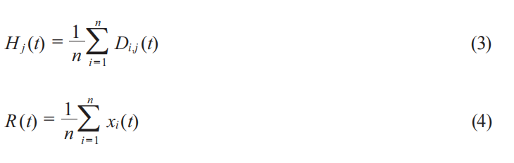
where H_j(t) denotes the final decomposed components obtained by EEMD, and R(t) represents the final residual component.

2.2 Principle of temporal fusion transformer (TFT)

The Temporal Fusion Transformer (TFT) is a valuable deep learning framework that has proven to be more reliable and effective in solving various intricate time-series problems, such as photovoltaic power prediction and financial market volatility forecasting [8,9]. In comparison to traditional statistical models such as ARIMA or classical recurrent neural networks such as LSTM, TFT uses gating mechanisms and self-attention structures to learn the dynamics of multi-scale time-varying dynamics and enhances the interpretability and consistency of non-stationary epidemiological processes much more.

Figure 1 shows the detailed TFT architecture that consists of variable selection networks (VSN), gated residual networks (GRN), and interpretable multi-head attention mechanisms. The model processes both known and observed inputs through specialized modules, enabling it to dynamically select the most relevant features at each time step, encode covariates, and model past and present inputs effectively. Local temporal interactions are learnt through sequence-to-sequence layers and long term interaction through the multi head attention. Hierarchical modeling of multi-source features in TFT gives features interpretable relative significance and interaction of input variables, which minimizes the black-box quality of deep neural networks [10].

Temporal Fusion Transformer (TFT) uses Gated Residual Network (GRN) as one of the important nonlinear feature transformation modules used to make feature mapping and filtering of information. GRN is able to perform this additional task through the addition of gated linear units (GLU) with residual connections, to maintain model expressiveness and stabilize training. The computation of GRN is defined as

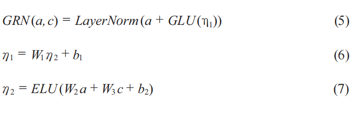
where a denotes the primary input, c represents contextual information, and W and b are learnable parameters.

To capture long-term temporal dependencies, TFT introduces the Interpretable Multi-head Attention (IMHA) mechanism to model interactions between different time steps. The core attention computation can be expressed as:

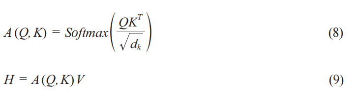
Where Q, K, and V denote the query, key, and value matrices, respectively, and d_k is the feature dimension.

Furthermore, TFT adopts quantile forecasting to estimate prediction intervals and quantify predictive uncertainty. The model is trained by minimizing the quantile loss function:

where y is the observed value, is the predicted value, and q denotes the quantile level. By jointly optimizing multiple quantile losses, the model can generate prediction intervals at different confidence levels.

2.3 Description of the RG-EEMD-TFT model architecture

To address the non-stationary and multi-scale characteristics of influenza surveillance time series, this study proposes a reconstruction-grouped EEMD and Temporal Fusion Transformer framework (RG-EEMD-TFT) for influenza trend forecasting. EEMD is first applied to decompose weekly influenza-like illness (ILI%) data into several intrinsic mode functions (IMFs) and a residual component. This decomposition is necessary to disentangle the complex, multi-scale dynamics of ILI time series, which are often poorly captured by conventional models. By separating these temporal components, EEMD enables subsequent models to capture patterns at different frequencies more effectively [11].

However, directly using all IMF components as model inputs can introduce redundancy and unnecessary complexity. To further recombine the decomposed IMFs according to the dominating frequencies, a reconstruction grouping (RG) strategy is further proposed. In particular, the IMFs are totally summed up and rebuilt into three representative parts that relate to the high-frequency fluctuations, seasonal changes and long-term tendencies. The reconstruction process minimizes redundancy in features, and at the same time, it maintains key multi-scale features of the original sequence. The reconstructed components are then standardized and aligned to form a compact, multi-scale input representation for the forecasting model.

Thereafter, the Temporal Fusion Transformer (TFT) is used to predict the sequences rebuilt. TFT is especially suitable for processing the multi-scale components generated by the RG-EEMD process since its gating processes, choice of variables networks, and interpretable attention networks have the ability to dynamically select the most informative temporal cues in one step. This allows long term trends, seasonal variations and high frequency variations to be observed by the model at the same time making the model more interpretable.

In the course of the training, the NNI hyperparameter optimization framework is used to optimize important TFT parameters automatically to enhance prediction accuracy and generalization. The trained RG-EEMD-TFT model provides multi-week ILI predictions, and interpretable analysis according to the weights of attention and feature importance, which can inform dynamic decision-making in public health practice. The overall architecture of the proposed model is illustrated in Figure 2.

3.1 Data source

The influenza-like illness (ILI) data used in this study were obtained from the FluView platform on the official website of the Centers for Disease Control and Prevention (CDC), where surveillance data are reported weekly. In this study, weekly ILI surveillance data from the state of Colorado in the United States were selected as the dataset. To avoid atypical disturbances in natural influenza transmission caused by large-scale non-pharmaceutical interventions and competitive virus circulation following the outbreak of COVID-19, weekly ILI data from week 1 of 2011 to week 52 of 2019 were used for model development and evaluation [12]. The ILI visit percentage (ILI%) was used as the core analytical indicator and is calculated as follows:

Figure 3 shows the weekly ILI% trend in Colorado, USA, from 2011 to 2019, indicating that influenza activity exhibits a typical winter-concentrated outbreak pattern, mainly occurring from week 45 of each year to week 10 of the following year.

3.2 Evaluation indicators

In order to measure the prediction error of the model, in this paper root mean square error (RMSE), mean absolute error (MAE) and mean absolute percentage error (MAPE) are used as the fundamental evaluation measures. Of the above, MAE is most intuitively the average size of errors in prediction, MAPE is a scale-invariant index of relative error, allowing it to be compared across data sets, whereas RMSE makes larger errors more heavily penalized by the squared terms and thus measures the distribution of the spread between forecast and observed outcomes. The relevant formulas are as follows:

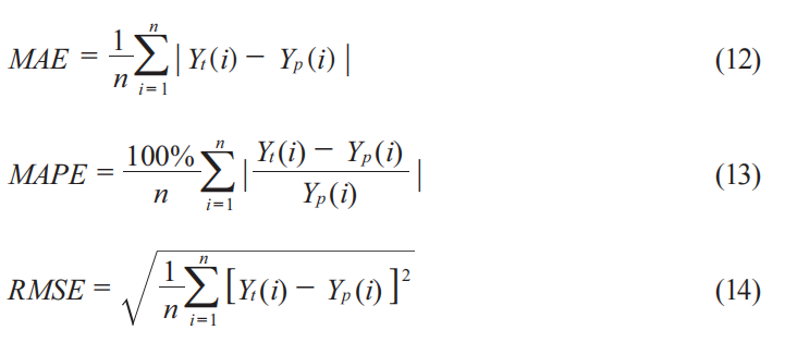
Here, Y_t(i) denotes the observed ILI% value in week i, and Y_p(i) denotes the predicted ILI% value in week i, for each of the above metrics, lower values indicate better predictive performance of the model.

3.3 Ensemble empirical mode decomposition (EEMD) process

This study uses weekly influenza-like illness (ILI) data from Week 1 of 2011 to Week 52 of 2019 for model development and divides the dataset chronologically; specifically, data from Week 1 of 2011 to Week 52 of 2017 (364 weeks) are used as the training set, data from Week 1 of 2018 to Week 52 of 2018 (52 weeks) are used as the validation set, and data from Week 1 of 2019 to Week 52 of 2019 (52 weeks) are used as the test set.

In this study, a range of Gaussian (0.1 to 0.4) white noise amplitudes was tested in EEMD trials to mitigate mode mixing while preserving the temporal structure. The best amplitude was found to be 0.2 times the standard deviation of the original series and an ensemble size of 100 was selected to reach a compromise on both the stability of the decomposition and the cost of computation. The eight intrinsic mode functions (IMF1-IMF8) and one residual component estimated by applying EEMD to weekly influenza-like illness (ILI%) data between Week 1 of 2011 and Week 52 of 2017 (Figure 4) decomposed the original nonlinear and non-stationary time-dependent data, which together represent the multi-scale temporal structure of the original ILI% time series.

Assuming a weekly temporal resolution and denoting week t as a time step, the original ILI% time series can be expressed as follows after EEMD decomposition:

3.4 The reconstruction grouping (RG) process

To further characterize the temporal features of the decomposed components, a Hilbert spectral analysis of each of the IMFs was conducted and of the residual component. The average time-resolved frequency of each component was computed to represent its prevailing scale of oscillation, and the energy of each component was also computed in order to determine the proportionate contribution of each component to the original signal.

The average instantaneous frequency, as shown in Figure 5A, reduces gradually as the IMF index increases, i.e., from IMF1 to IMF8, indicating a clear shift toward lower-frequency oscillations. IMF1 and IMF2 have the highest frequencies that are equivalent to short-term stochastic variations and local irregularities of the influenza time series. IMF3-IMF5 are intermediate frequency ranges, which relate to periodic oscillations in line with the seasonal influenza regional cycles. Conversely, IMF6-IMF8 and the residual part have very low mean frequencies, which constitute the long-term dynamics of evolution of the incidence of influenza.

Figure 5B also indicates the validity of the multi-scale structure of the decomposed ILI% series, as reflected by the energy distribution. Although the periodic variations associated with seasonal influenza epidemics are mainly contained in the intermediate-frequency components IMF3-IMF5, a substantial proportion of the signal energy is concentrated in the lower-frequency components IMF7 and IMF8. This implies that long-term variation and slowly changing background trends account for a large share of the overall dynamics of the influenza time series. The residual component also retains a relatively high energy proportion, further confirming that an important part of the original ILI% signal lies in the low-frequency domain. Combined with IMF7 and IMF8, the residual term captures the smooth background evolution and long-term trend information of influenza activity. This result supports grouping these components into the trend-related representation in the subsequent reconstruction stage.

With such spectral properties, the reconstruction grouping (RG) strategy was used to combine the decomposed elements into three meaningful groups, namely, the high-frequency components (IMF1-IMF2), the seasonal components (IMF3-IMF5), and the trend components (IMF6-IMF8 along with the residual). The results of the reconstruction are demonstrated in Figure 6. This grouping strategy not only maintains the prevailing multi-scale information of the original signal, but also minimizes redundancy between individual IMFs, hence it provides structured inputs in the latter TFT-based prediction model.

3.5 Comparative experiments of discrete wavelet transform

To highlight the effectiveness of RG-EEMD, we introduced the discrete wavelet transform (DWT) as a representative comparative decomposition method. DWT is a widely used multi-resolution analysis technique that decomposes a signal into low-frequency approximation components and high-frequency detail components at different scales, thereby separating long-term trend information from local fluctuation patterns [13]. Previous studies have demonstrated that wavelet-based methods have been successfully applied to the multiscale analysis, outbreak detection, and dynamic modeling of influenza-related time series, making DWT a reasonable comparative approach for evaluating the advantages of EEMD-based decomposition [14].

In this study, the original ILI% series was decomposed using a three-level discrete wavelet transform (DWT) implemented in Python through the PyWavelets (pywt) library. The Daubechies 4 (db4) wavelet was selected because it is widely used in non-stationary biomedical and epidemiological time-series analysis and is effective in separating smooth trend components from short-term fluctuations. The decomposition produced one low-frequency approximation component (A3) and three high-frequency detail components (D3, D2, and D1), as illustrated in Figure 7. Among these components, A3 mainly preserves the long-term trend and overall epidemic level of the original series, D3 and D2 capture medium- and low-frequency fluctuation patterns, while D1 primarily represents short-term rapid variations and partial noise information. This process allows the complex ILI% sequence to be represented as a superposition of components across different frequency scales, enabling subsequent prediction models to learn long- and short-term patterns more effectively.

3.6 Model parameter selection and training

Following the use of the RG-EEMD decomposition, the original influenza series were rebuilt into three illustrative elements high-frequency, seasonal and trend sequences. The TFT model took these reconstructed components as the observed covariates, to give multi-scale temporal information. The weekly ILI percentage is the forecasting variable of the task. The model uses these reconstructed components as explanatory variables to predict the original ILI% series, allowing it to learn the contribution of different temporal scales to influenza dynamics.

Because predictive effectiveness of the Temporal Fusion Transformer (TFT) and Long Short-Term Memory (LSTM) models is very sensitive to the choice of hyperparameter combinations, manual search is often inefficient and unsystematic. Thus, the proposed study introduces the automated hyperparameter optimization framework NNI, which employs global hyperparameter optimization. NNI can effectively search for the optimal parameter settings in non-stationary influenza time series through the built-in tuning algorithms it provides, to enhance the generalization of the model and its robustness against these non-stationary dynamics [15,16].

This study adopts a forecasting horizon of four weeks. The rationale behind this design is the fact that influenza outbreaks are usually characterized by sudden outbreaks; hence, decisions based solely on one-week forecasts may be insufficient for timely public health responses. Conversely, a month of forecasting timeframe will have a realistic decision-making window for the public health officials in the region like resource allocation, adjusting to a vaccination program, and alerting to the presence of an epidemic in the region [17,18]. The final results of the RG-EEMD-TFT model hyperparameters in this study have been determined after the repeated runs of the related model in the NNI framework, which are summarized in Table 1.

To avoid information leakage from global decomposition, EEMD-based preprocessing during the validation and test stages was performed in a strictly chronological manner. Specifically, for each forecast origin, only the observed ILI series up to that time point, denoted as X_1:t={x₁,x₂,…,x_t}, was used for decomposition. EEMD was applied to X_1:t to obtain the corresponding IMF components and residual term, after which the decomposed components were analyzed and reconstructed into high-frequency, seasonal, and trend signals based solely on the information contained in the historical segment X_1:t. The reconstructed components within the most recent encoder window were then used as input to the TFT model to generate forecasts for the next 4 weeks, ensuring that the evaluation was free from look-ahead bias.

All the experiments were performed on a workstation with an Intel Core i7-12700KF processor, 32 GB of Random Access Memory, and an NVIDIA GeForce RTX 3060 graphics card (12 GB VRAM). The experiments were conducted using Python 3.10 and PyTorch, with PyTorch used as the deep learning framework for building and training the Temporal Fusion Transformer (TFT). To reduce the influence of randomness in deep learning training, all deep learning models were evaluated through repeated experiments under different random seeds. Specifically, each model was independently trained and tested 10 times under the same chronological data split, hyperparameter settings, and training procedure, and the final results were reported as the mean ± standard deviation of MAE, MAPE, and RMSE on the test set.

The ARIMA model was another baseline model presented by this study in the comparative experiments. Due to the fact that the ARIMA model is a classical univariate time series model, the historical ILI% data were the only input variables that were utilized in this study. Parameter validation for the ARIMA model is typically conducted using two approaches. The first approach involved applying first-order and seasonal differencing to the ILI% series to remove trends and account for its 52-week annual cycle, thereby stabilizing the data. Subsequently, by examining the autocorrelation function (ACF) and partial autocorrelation function (PACF) plots of the differenced series (see Figure 8), the cutoff and tailing-off characteristics are used to preliminarily determine the range of model orders [19]. The second approach employed the automated auto_arima function from Python's pmdarima library (originally a Python port of the R language forecast package). This method automatically tested different combinations of the ARIMA(p,d,q)(P,D,Q)_m parameters within a given search range and selected the optimal model based on goodness-of-fit criteria, such as the Akaike Information Criterion (AIC) [20]. Based on a comprehensive analysis of the two aforementioned approaches, this study ultimately determined the parameters of the seasonal ARIMA model as ARIMA(2,1,1)(1,1,1)52, which were then used for subsequent influenza trend forecasting.

3.7 Results

To evaluate the effectiveness of the proposed RG-EEMD-TFT model for influenza trend forecasting, a multi-stage comparative experiment was conducted. Initially, we compared our proposed approach against traditional statistical and deep learning baselines that did not employ signal decomposition. To ensure the rigor of the results and eliminate the interference of random initialization, all deep learning models were executed 10 times with different random seeds. As shown in Table 2, the traditional ARIMA model yields relatively high MAPE (17.223%) and RMSE (0.789), as it struggles to process the nonlinear and non-stationary properties of influenza surveillance data. In contrast, deep learning models such as LSTM and TFT, as well as the recent state-of-the-art (SOTA) models DLinear and PatchTST, achieve higher predictive accuracy. Specifically, PatchTST achieves the best performance among baselines (MAE=0.551±0.014), benefiting from its patching mechanism which effectively extracts local semantic information from the time series.

We further investigated the impact of signal decomposition on forecasting performance. As shown in Table 3, hybrid models incorporating decomposition techniques significantly outperform their single-model counterparts. Comparing DWT-TFT and EEMD-TFT, the EEMD-based approach demonstrates superior gains. This superiority stems from the fact that Discrete Wavelet Transform (DWT) relies heavily on the selection of wavelet bases and predefined frequency partitioning. In contrast, EEMD is an adaptive, data-driven method that decomposes the ILI sequence into various Intrinsic Mode Functions (IMFs) based on the local characteristic time scales of the data itself, thereby capturing complex non-stationary dynamics and seasonal fluctuations more accurately.

Finally, to verify the role of the RG strategy in reducing information redundancy, we integrated it into various deep learning architectures. As presented in Table 4, incorporating the RG strategy consistently yields further reductions in forecasting error. Ultimately, the proposed RG-EEMD-TFT model achieved the best overall performance (MAE=0.318, MAPE=8.012%). This success is attributed to the RG strategy's ability to consolidate multiple IMFs into high-frequency, seasonal, and trend components. This reduction in dimensionality attenuates noise while enabling the Transformer-based TFT architecture to concentrate on the dominant temporal structures of influenza activity. Furthermore, a Diebold-Mariano test confirmed that the performance improvements of RG-EEMD-TFT over other SOTA models are statistically significant (p<0.05), validating its superior competitiveness in influenza forecasting.

Figure 9 illustrates the rolling forecast performance of some models on the 2019 test set. The RG-EEMD-TFT model is more accurate amongst the others. In addition, the p10 to p90 quantile prediction intervals generated by the RG-EEMD-TFT model widen adaptively with increasing influenza intensity, effectively reflecting the stochastic uncertainty during outbreak peaks. This feature highlights the model's robustness and its value for public health risk early warning and decision support.

3.8 Interpretability analysis of the TFT model

In addition, the Variable Selection Network (VSN) embedded in the TFT architecture was used to compare the feature attribution patterns of the EEMD-TFT and RG-EEMD-TFT models (Figure 10). For the original EEMD-TFT model, variable importance was distributed across multiple IMF components, with greater importance weights assigned to IMF7, IMF4, IMF5, and IMF8. This indicates that the model mainly relied on low-frequency trend-related and seasonal components. The RG-EEMD-TFT model exhibited a more concentrated and structurally compact attribution pattern after reconstruction grouping. Specifically, the trend component had the highest importance weight (58.21%), followed by the seasonal component (34.87%), whereas the high-frequency component accounted for only 6.92%. Compared with the IMF-level attribution pattern of the original EEMD-TFT model, this result suggests that the reconstruction grouping strategy enables the model to focus more directly on the dominant low-frequency and periodic structures of influenza activity, while further suppressing the influence of short-term stochastic disturbances and noise.

The results demonstrate that decomposition-based hybrid models consistently outperform their non-decomposition counterparts, confirming that signal decomposition effectively addresses the non-stationary and multi-scale characteristics of ILI series. Compared with DWT, EEMD provides superior predictive performance, as its adaptive, data-driven decomposition is more suitable for capturing the intrinsic temporal dynamics of influenza activity. Under the same decomposition framework, TFT consistently outperforms LSTM and recent SOTA models like DLinear and PatchTST, suggesting that its variable selection and multi-head attention mechanisms are better suited to integrating complex, multi-component inputs.

Furthermore, the implementation of the reconstruction grouping (RG) strategy yields additional performance gains across all architectures, particularly for RG-EEMD-TFT. This indicates that consolidating decomposed IMFs into high-frequency, seasonal, and trend representations effectively reduces information redundancy and enhances the compactness of multi-scale representations. Beyond point estimates, the RG-EEMD-TFT model also exhibits excellent probabilistic forecasting capabilities; quantitative assessments yield a PICP of 0.842 and a PINAW of 0.126, proving that the proposed framework provides statistically reliable coverage with high interval sharpness.

In this study, an RG-EEMD-TFT framework was proposed for influenza forecasting. By combining EEMD decomposition, reconstruction grouping, and TFT-based temporal modeling, the proposed method achieved the best predictive performance among all compared models. indicating that the integration of adaptive decomposition, feature reconstruction, and temporal fusion learning is a promising approach for influenza forecasting. This framework may provide useful methodological support for epidemic trend monitoring and public health decision-making.

Author contributions

Defu Lin participated in data collection and experiment execution, while Zhaoxue Chen provided guidance on experimental design.

Funding

This research received no external funding.

Data availability

The data presented in this study are authentic and reliable.

Ethics approval and consent to participate

Not applicable (this study did not involve any procedures requiring ethical review).

Consent for publication

The submitted manuscript has not been published elsewhere (except in the form of an abstract or a conference presentation) and is not currently under consideration for publication by any other journal.

Competing interests

The authors declare no potential conflicts of interest with respect to the research, authorship, or publication of this article.

Acknowledgements

Not applicable.

[1] Troeger CE, Blacker BF, Khalil IA, Zimsen SRM, Albertson SB, Abate D, et al. Mortality, morbidity, and hospitalisations due to influenza lower respiratory tract infections, 2017: An analysis for the Global Burden of Disease Study 2017. Lancet Respir Med. 2019 Jan;7(1):69-89. https://doi.org/10.1016/S2213-2600(18)30496-X

[2] Li G, Li Y, Han G, Jiang C, Geng M, Guo N, et al. Forecasting and analyzing influenza activity in Hebei Province, China, using a CNN-LSTM hybrid model. BMC Public Health. 2024 Aug 12;24(1):2171. https://doi.org/10.1186/s12889-024-19590-8

[3] Yang CT, Chen YA, Chan YW, Lee CL, Tsan YT, Chan WC, et al. Influenza-like illness prediction using a long short-term memory deep learning model with multiple open data sources. J Supercomput. 2020;76(12):9303-9329. https://doi.org/10.1007/s11227-020-03182-5

[4] Javanian M, Barary M, Ghebrehewet S, Koppolu V, Vasigala V, Ebrahimpour S. A brief review of influenza virus infection. J Med Virol. 2021 Aug;93(8):4638-4646. https://doi.org/10.1002/jmv.26990

[5] Zhang G, Patuwo BE, Hu M. Forecasting with artificial neural networks: The state of the art. Int J Forecasting. 1998;14(1):35-62. https://doi.org/10.1016/S0169-2070(97)00044-7

[6] Li Y, Gao S, Zhang S, He H, Xian P, Yuan C. The baseline wander correction based on the improved ensemble empirical mode decomposition (EEMD) algorithm for grounded electrical source airborne transient electromagnetic signals. Geosci Instrum Method Data Syst. 2020;9(2):443-450. https://doi.org/10.5194/gi-9-443-2020

[7] Luo L, Zhang Y, Dong W, Zhang J, Zhang L. Ensemble empirical mode decomposition and a long short-term memory neural network for surface water quality prediction of the Xiaofu River, China. Water. 2023;15(8):1625. https://doi.org/10.3390/w15081625

[8] López Santos M, García-Santiago X, Echevarría Camarero F, Blázquez Gil G, Carrasco Ortega P. Application of temporal fusion transformer for day-ahead PV power forecasting. Energies. 2022;15(14):5232. https://doi.org/10.3390/en15145232

[9] Hartanto S, Gunawan AAS. Temporal fusion transformers for enhanced multivariate time series forecasting of Indonesian stock prices. Int J Adv Comput Sci Appl. 2024;15(7):140-148. https://doi.org/10.14569/IJACSA.2024.0150713

[10] Lim B, Arık SÖ, Loeff N, Pfister T. Temporal fusion transformers for interpretable multi-horizon time series forecasting. Int J Forecasting. 2021;37(4):1748-1764. https://doi.org/10.1016/j.ijforecast.2021.03.012

[11] Ha J, Lee S, Jeong S, Chung D. Methodology for advanced time series demand forecasting: A hybrid model of decomposition and deep learning. Intell Syst Appl. 2025;27:200540. https://doi.org/10.1016/j.iswa.2025.200540

[12] Feng L, Zhang T, Wang Q, Xie Y, Peng Z, Zheng J, et al. Impact of COVID-19 outbreaks and interventions on influenza in China and the United States. Nat Commun. 2021 May 31;12(1):3249. https://doi.org/10.1038/s41467-021-23440-1

[13] Zhang Z. The improvement of the discrete wavelet transform. Mathematics. 2023;11(8):1770. https://doi.org/10.3390/math11081770

[14] Agyemang EF. A gaussian process regression and wavelet transform time series approaches to modeling influenza A. Comput Biol Med. 2025 Jan;184:109367. https://doi.org/10.1016/j.compbiomed.2024.109367

[15] Fra V. Application-oriented automatic hyperparameter optimization for spiking neural network prototyping. arXiv [preprint]. 2025 [cited 2026 Mar 1]. Available from: https://doi.org/10.48550/arXiv.2502.12172

[16] Gridin I. Automated deep learning using neural network intelligence: Develop and design pytorch and tensorflow models using Python. Springer; 2022. https://doi.org/10.1007/978-1-4842-8149-9

[17] Reich NG, Brooks LC, Fox SJ, Kandula S, McGowan CJ, Moore E, et al. A collaborative multiyear, multimodel assessment of seasonal influenza forecasting in the United States. Proc Natl Acad Sci U S A. 2019 Feb 19;116(8):3146-3154. https://doi.org/10.1073/pnas.1812594116

[18] Lutz CS, Huynh MP, Schroeder M, Anyatonwu S, Dahlgren FS, Danyluk G, et al. Applying infectious disease forecasting to public health: A path forward using influenza forecasting examples. BMC Public Health. 2019 Dec 10;19(1):1659. https://doi.org/10.1186/s12889-019-7966-8

[19] Alzahrani SM, Saadeh R, Abdoon MA, Qazza A, Guma FE, Berir M. Numerical simulation of an influenza epidemic: Prediction with fractional SEIR and the ARIMA model. Appl Math Inf Sci. 2024;18(1):1-12. https://doi.org/10.18576/amis/180101

[20] Tsan YT, Chen DY, Liu PY, Kristiani E, Nguyen KL, Yang CT. The prediction of influenza-like illness and respiratory disease using LSTM and ARIMA. Int J Environ Res Public Health. 2022 Feb 7;19(3):1858. https://doi.org/10.3390/ijerph19031858